The EM algorithm

For many models in machine learning and statistics, computing the ML or MAP parameter estimate is easy provided we observe all the values of all the relevant random variables, i.e., if we have complete data. However, if we have missing data and/or latent variables, then computing the ML/MAP estimate becomes hard. One approach is to use a generic gradient-based optimizer to find a local minimum of the negative log likelihood or NLL, given by

However, we often have to enforce constraints, such as the fact that covariance matrices must be positive definite, mixing weights must sum to one, etc., which can be tricky. In such cases, it is often much simpler (but not always faster) to use an algorithm called expectation maximization, or EM for short. This is a simple iterative algorithm, often with closed-form updates at each step. Furthermore, the algorithm automatically enforce the required constraints. EM exploits the fact that if the data were fully observed, then the ML/ MAP estimate would be easy to compute. In particular, EM is an iterative algorithm which alternates between inferring the missing values given the parameters (E step), and then optimizing the parameters given the “filled in” data (M step). We give the details below, followed by several examples.

Let $\bold x_i$ be the visible or observed variables in case $i$, and let $\bold z_i$ be the hidden or missing variables. The goal is to maximize the log likelihood of the observed data:

Unfortunately this is hard to optimize, since the log cannot be pushed inside the sum.

EM gets around this problem as follows. Define the complete data log likelihood to be

Let the marginal likelihood as

The complete data log likelihod cannot be computed. So lets define the expected complete data log likelihood as follows:

$Q$ is called the auxiliary function. The expectation is taken wrt the old parameters, $\theta^{(t-1)}$, and the observed data $\mathcal{D}$. The goal of the E step is to compute $Q(\theta, \theta^{(t-1)})$ or rather, the terms inside of it which the MLE depends on; these are known as the expected sufficient statistics or ESS. In the M step, we optimize the Q function wrt $\theta$:

To perform MAP to avoid overfitting:

We could easily maximize

E-step: $q^{(t+1)} = \arg\max_q F(q,\theta^{(t)})$. In class label problems, the E-step is to estimate the responsibility of one data belongs to that class label. M-step: $\theta^{(t+1)} = \arg\max_\theta (F(q^{(t+1)},\theta)$ Using the new class label, we may choose a new parameter $\theta$ to maximize the likelihood.

Taking maxture of Gausians as an example, the expected complete data log likelihood is given by

where $r_ik \triangleq p(z_i = k | \bold x_i, \theta^{(t-1)})$ is the responsibility that cluster $k$ takes for data point $i$. This is computed at the E step:

M step: in the M step, we optimize Q wrt $\pi$ and the $\theta_k$. For $\pi$, we obviously have

Which is the averaged responsibility for cluster $k$. However, the M step will have no regard to $\pi$. and

This is just a weighted version of the standard problem of computing the MLEs of an MVN and the new parameter estimate is given by

import numpy as np
def gaussian_point_generator(mu:list,sigma:list,n:int):
    return list(zip(np.random.normal(mu[0], sigma[0], n), np.random.normal(mu[1], sigma[1], n)))


class GaussianParameter:
    def __init__(self, mu:list,sigma:list, cov=0):
        self.mu = mu
        self.sigma = sigma
        self.cov=cov

    def __repr__(self):
        return "".format(self.mu, self.sigma)

    def plot(self, ax):
        m = np.array([[self.mu[0]],[self.mu[1]]])
        cov = np.array(self.sigma)
        cov_inv = np.linalg.inv(cov)  # inverse of covariance matrix
        cov_det = np.linalg.det(cov)  # determinant of covariance matrix
        x = np.linspace(-20,20)
        y = np.linspace(-20,20)
        X,Y = np.meshgrid(x,y)
        coe = 1.0 / ((2 * np.pi)**2 * cov_det)**0.5
        Z = coe * np.e ** (-0.5 * (cov_inv[0,0]*(X-m[0])**2 + (cov_inv[0,1] + cov_inv[1,0])*(X-m[0])*(Y-m[1]) + cov_inv[1,1]*(Y-m[1])**2))
        ax.contour(X,Y,Z)

    def p(self, point):
        return np.array((1 / 2 * np.pi * np.power(np.linalg.det(np.matrix(self.sigma)), 0.5) ) * np.exp( -1/2 * (np.matrix(np.array(self.mu)) - np.matrix(np.array(point))) * np.matrix(self.sigma) *  (np.matrix(np.array(self.mu)) - np.matrix(np.array(point))).T))[0][0]

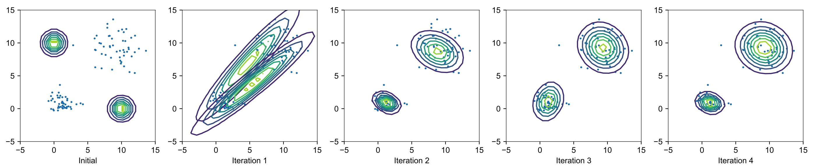
    init_gaussian_parameter = [GaussianParameter([0,10], [[1,0],[0,1]]), GaussianParameter([10,0], [[1,0],[0,1]])]

    points = gaussian_point_generator([1,1], [1,1],50) + gaussian_point_generator([9,9], [2,2],50)

def iterate(axis):
    r = [[], []]
    for i in points:
    for j in range(2):
        r[j].append(init_gaussian_parameter[j].p(i))

    r[0], r[1] = np.array(r[0]) / (np.array(r[0]) + np.array(r[1])), np.array(r[1]) / (np.array(r[0]) + np.array(r[1]))
    r[0] = np.array(list(map(lambda x:0 if np.isnan(x) else x, r[0])))
    r[1] = np.array(list(map(lambda x:0 if np.isnan(x) else x, r[1])))
    new_mu = [np.array([0,0]), np.array([0,0])]
    for j in range(2):
    for ind,i in enumerate(points):
        new_mu[j] = new_mu[j] + r[j][ind] * np.array(i)
    new_mu[j] = new_mu[j] / np.sum(r[j])

    new_sigma = [np.array([[0,0], [0,0]]), np.array([[0,0], [0,0]])]
    for j in range(2):
    for ind,i in enumerate(points):
        new_sigma[j] = new_sigma[j] + r[j][ind] * np.matrix(i).T * np.matrix(i)
    new_sigma[j] = new_sigma[j] / np.sum(r[j])
    new_sigma[j] = new_sigma[j] - np.matrix(new_mu[j]).T * np.matrix(new_mu[j])
    init_gaussian_parameter[j].mu = np.array(new_mu[j])
    init_gaussian_parameter[j].sigma = np.array(new_sigma[j])
    init_gaussian_parameter[0].plot(axis)
    init_gaussian_parameter[1].plot(axis)
                    

The result gives